The LH Strip Detection & Quantification System
This case documents a production biosensing algorithm used to extract quantitative LH (Luteinizing Hormone) values from user-uploaded smartphone photos of ovulation test strips.
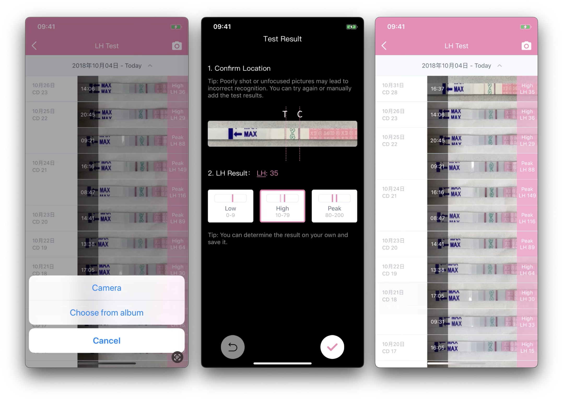 Unlike lab-controlled imaging, this system operates under fully unconstrained conditions: arbitrary backgrounds, lighting variations, multiple strips in one image, blur, partial occlusion, and heterogeneous user behavior. The core challenge is not only detection accuracy, but stability, explainability, and latency in a medical-adjacent context.
The final solution is a cascaded hybrid pipeline combining classical computer vision, feature-based machine learning, and deep learning — each used where it is strongest.
Problem Definition
Input
User-uploaded photo (full image or cropped)
Device: iOS / Android
No constraints on background, orientation, or light condition
Output
Quantitative LH value
Interpreted state (low / high / peak)
Detection metadata (line position, confidence, fallback path)
Core Constraints
Deterministic, explainable computation preferred over black-box prediction
Low latency suitable for mobile / near-real-time processing
Robustness against repeated capture, batch uploads, and noisy inputs
High recall is mandatory (false negatives are unacceptable)
System Overview
The system is intentionally hierarchical, prioritizing fast and deterministic methods first, and escalating to more powerful (but expensive) deep learning models only when necessary.
Full Image
	↓
[StripDetector] (Stage 1: Strip Region Detection)
	↓
Candidate Strip ROI
	↓
[AssayInspectorWrapper] (Stage 2-3: Assay Region Localization)
	|
	├─ [CVInspector] (OpenCV based fast path)
	|
	└─ [TfInspector] (Tensorflow DL based fallback)
	↓
Candidate Assay ROI
	↓
Refinement & LH calculation (Stage 4: Quantification)
Stage 1 — Strip Region Detection (HoG + SVM)
Goal: Locate ovulation test strip regions from a full, unconstrained image.
Why HoG + SVM
The target object is a long, thin rectangle with strong geometric priors.
Sliding-window HoG offers excellent performance per FLOP for this shape class.
Kernel SVM provides strong decision boundaries with limited data.
The strip region detection rate is stable at approximately 95%.
End-to-end CNNs were unnecessary at this stage and would increase latency and complexity.
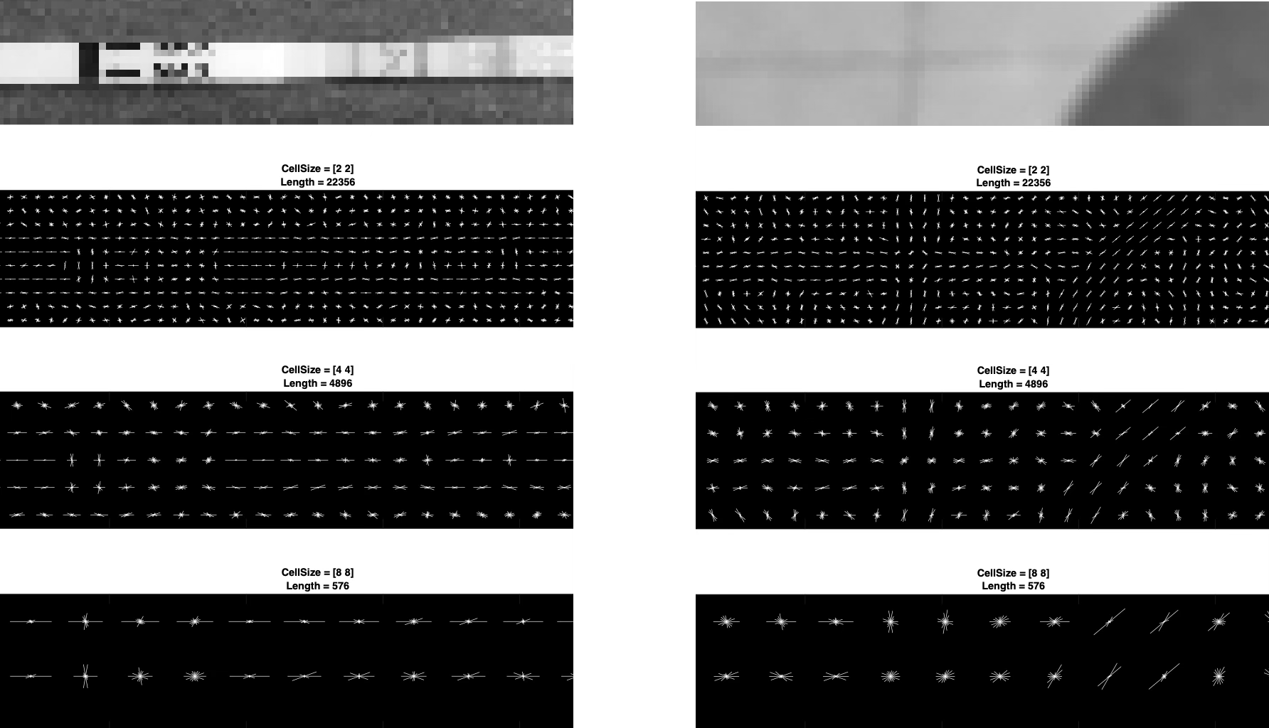 HoG Feature Visualization: Positive (Left) vs. Negative (Right) Samples at Different Pooling Sizes
Implementation Highlights
Image normalization to fixed aspect ratio (~7:1)
HoG feature extraction on standardized windows (e.g. 140×20)
Vertical sliding window optimized for typical strip placement
SVM scoring used to rank candidates
Non-Maximum Suppression (IoU-based) to remove overlapping detections
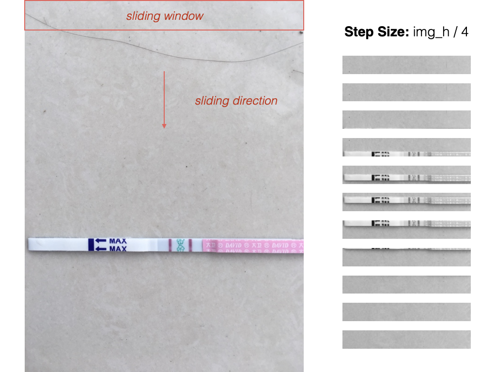
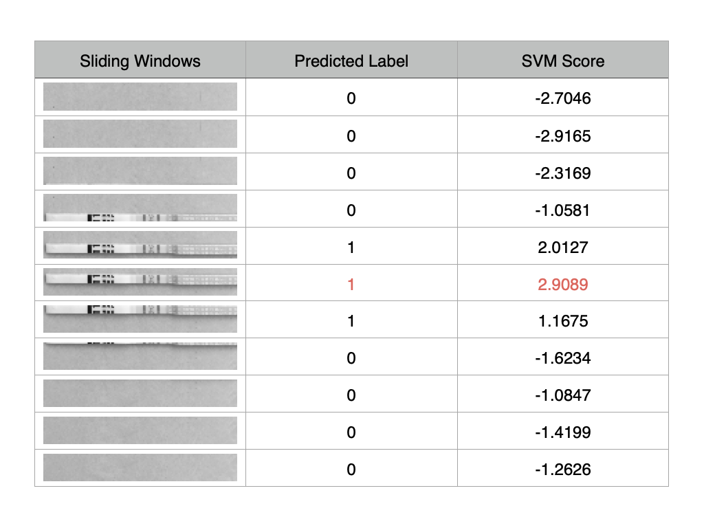 Sliding Window Visualization with SVM Scoring
Data Engineering (Critical)
Positive samples: human-verified strip crops
Negative samples: background patches extracted from real user images
Hard mining loop: false positives discovered on full images are iteratively added to the negative set
This hard-mining process dramatically reduced pathological false positives (e.g., pure black regions, strong linear textures).
Stage 2 — Assay Region Detection (OpenCV First)
Once a strip region is identified, the system attempts pure computer vision analysis.
Why CV First
Deterministic behavior
Pixel-level interpretability
No model loading overhead
Easier to debug and medically reason about
OpenCV Pipeline
Resize to standard width
Grayscale conversion
Gaussian blur (noise suppression)
Adaptive / OTSU thresholding
Morphological open/close
Contour detection
Polygon approximation + geometric filtering
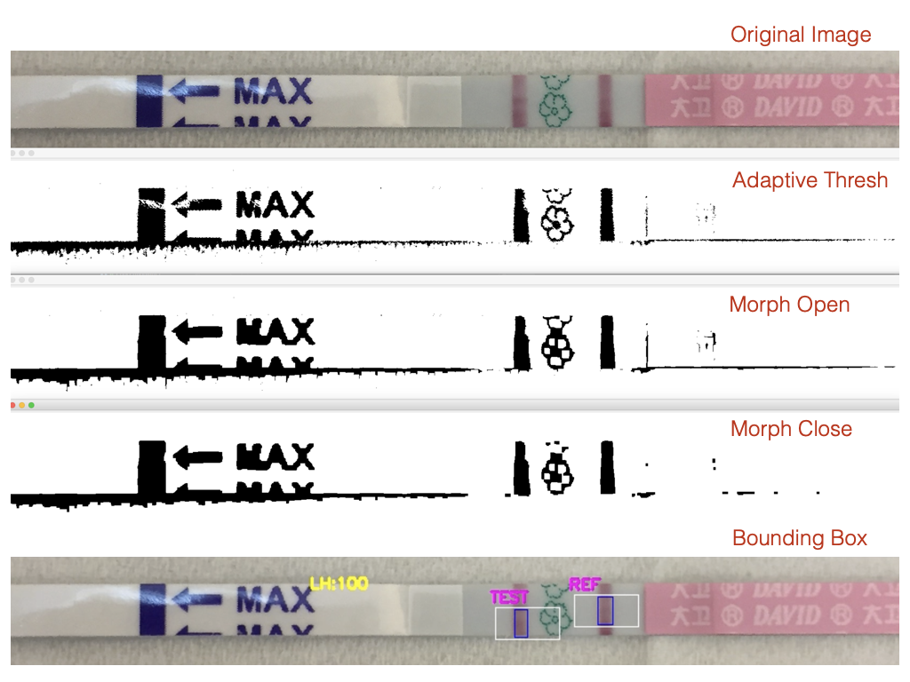 Visualization of Filtering Process for Assay Region Saliency
The goal is to detect:
Control line (or Reference line)
Test line
Their bounding rectangles and relative positions
Robustness Rules
The algorithm enforces multiple domain constraints:
Minimum density difference between line and background
Expected spatial relationship between control and test lines
Hue / RGB consistency checks when grayscale contrast is insufficient
Vertical expansion of line ROIs to handle broken or incomplete lines
Multi-scale retry when initial detection fails
When these checks pass, the system proceeds directly to LH calculation.
Stage 3 — Assay Region Fallback (TensorFlow Object Detection)
If OpenCV detection fails or is ambiguous, the system escalates, rather than guessing.
Trigger Mechanism
A wrapper layer (AssayInspectorWrapper) evaluates the OpenCV result:
If detection is confident → accept
If critical elements are missing or inconsistent → fallback
This is a contract-based decision, not parallel execution.
Deep Learning Role
TensorFlow object detector (SSD-style architecture)
Used only to localize the assay region
Optimized for recall: the TensorFlow fallback increases the overall LH detection rate from around 90% to over 95%
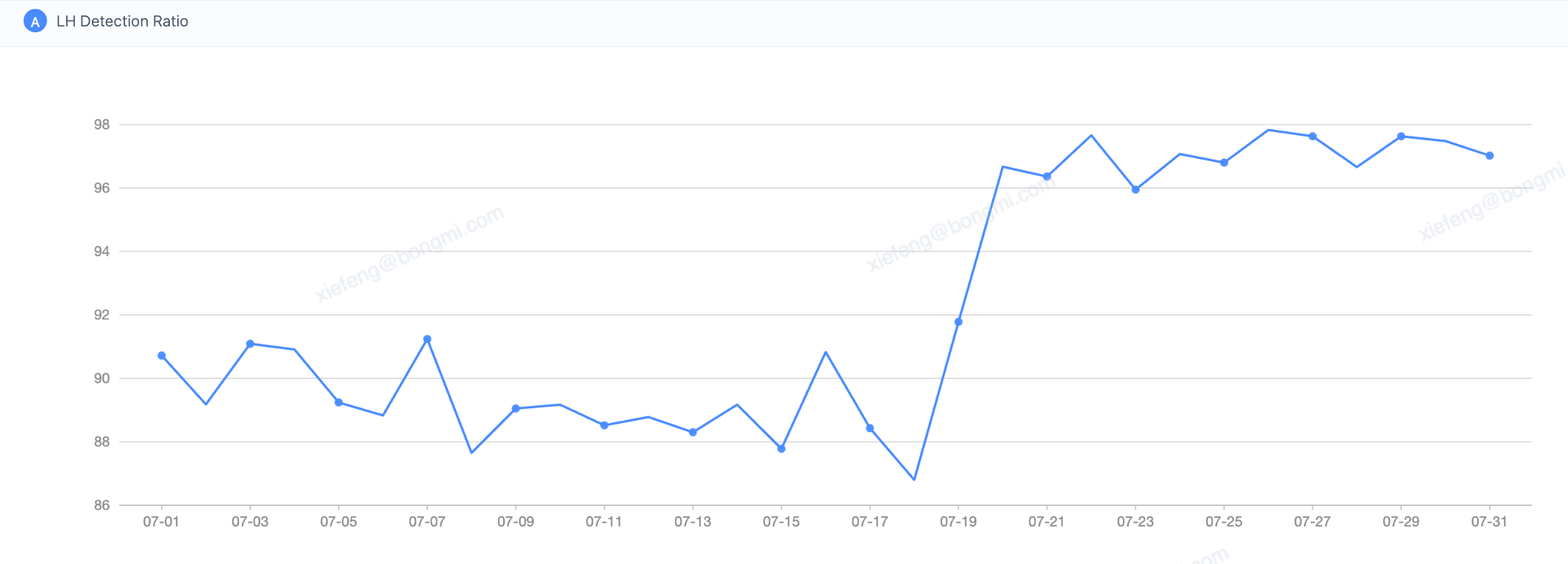 LH Detection Dashboard: Pre- vs. Post-TF Fallback Launch (Jul 18)
Importantly: The deep model does not compute LH values.
Instead, it recovers a reliable ROI, which is then passed back into the same OpenCV-based measurement logic (Stage 4). This preserves numerical consistency across fast and fallback paths.
Engineering Considerations
Singleton model loading (thread-safe)
Score thresholding and edge-box suppression
Color-space correction (BGR → RGB) to match training conditions
Stage 4 — LH Value Calculation (Deterministic CV)
The LH value calculation follows a straight-forward Non-ML process.
Algorithm
For both test and control lines:
Extract line ROI
Compute grayscale intensity distribution
Sort pixel values
Take the 25th percentile as line density
Subtract local background density
Final LH ratio:
LH = (TestLineDensity - TestBackground) /
     (ControlLineDensity - ControlBackground)
Stability Enhancements
Background sampled symmetrically around each line
Control line sanity checks (must exist and exceed threshold)
Expanded ROI coverage to avoid partial line artifacts
This approach prioritizes:
Repeatability across retakes
Device-independent behavior
Explainable numeric output
Evaluation & Tradeoffs
What Worked Well
Cascaded design significantly reduced average latency
Hard mining was more impactful than model choice
Classical CV remained the most reliable component under noise
DL fallback recovered edge cases without polluting normal flow
Known Tradeoffs
| Decision | Benefit | Cost |
|---|---|---|
| HoG + SVM | Fast, interpretable | Feature symmetry edge cases |
| CV-first strategy | Deterministic | Fragile under extreme lighting |
| DL as fallback | High recall | System complexity |
| Non-ML quantification | Stable, explainable | Requires careful heuristics |
Key Insights
Data quality and data engineering are foundational to building reliable biosensing systems.
Deep learning is a powerful tool, but its benefits are maximized when applied selectively—balancing model capacity, computational cost, and the structure of the problem rather than assuming end-to-end models are always the optimal choice.
Cascaded systems outperform monolithic models under real-world constraints.
In medical-adjacent applications, stability and explainability often outweigh marginal gains in raw accuracy.